For my first blog post I’ve decided to try out forecasting. Throughout my undergrad I came across forecasting many times. It was often very brief and conceptual, or the techniques was very basic. The goal is to apply the ARIMA model based on the last two years of daily returns of Danske Bank.
The ARIMA (Autoregressive integrated moving average) model consist of three components. These are an autoregressive, integraded and a moving average component. Below is a short breakdown of each component.
- AR is the autoregressive part which determines the number of previous periods are regressed on the variables. An AR(1) process can be denoted as: \[ y_{t}=c+\phi_{1} y_{t-1}+\varepsilon_{t} \] Where c is a constant, ϕ is the parameter and ε is the white noise.
- I is the differencing part. Differencing the change between to consecutive observations of the time series. A first order difference can be denoted as: \[ y_{t}^{\prime}=y_{t}-y_{t-1} \] Often the first order difference solves the issues of non-stationarity. However, it’s possible increase the order difference as one see fit.
- MA is the moving average. Instead using past values as a regressor like in the AR model, the MA model instead uses past error terms as a regressor. \[ y_{t}=c+\varepsilon_{t}+\theta_{1} \varepsilon_{t-1} \] The expected value is the constant c, the error term of time t and parameter ϕ multiplied by the error term of the previous period.
The number of lags and differences are denoted by p, d, q i. An ARIMA with one lag in both the autoregression and moving average with second order differencing would be called ARIMA(1,2,1).
To do the actual forecasting we are going to use the following packages in R:
library(quantmod)
library(tseries)
library(timeSeries)
library(forecast)
library(xts)
library(lmtest)
Data Preparation
Time to pull the data. This line of code pulls daily prices including volume.
getSymbols('DANSKE.CO', from='2017-08-01', to='2019-08-01', src = 'yahoo')I’m only going to use the adjusted close price. I simply reassign the Dansk Bank variable to only contain the adjusted close data.
DANSKE.CO <- DANSKE.CO[,4]Next I’m transforming the prices by taking the log. This can help achieve lower variance before the differencing. Furthermore, much finance literature often assumes prices are log-normal distributed and I’m no position to question the status quo.
DANSKE.CO <- log(DANSKE.CO)Finally I’m interested in the log-returns not log-price.
DANSKE.CO <- diff(DANSKE.CO, lag=1)
DANSKE.CO <- DANSKE.CO[!is.na(DANSKE.CO)] #Removes the first row since it does not contain the daily return.
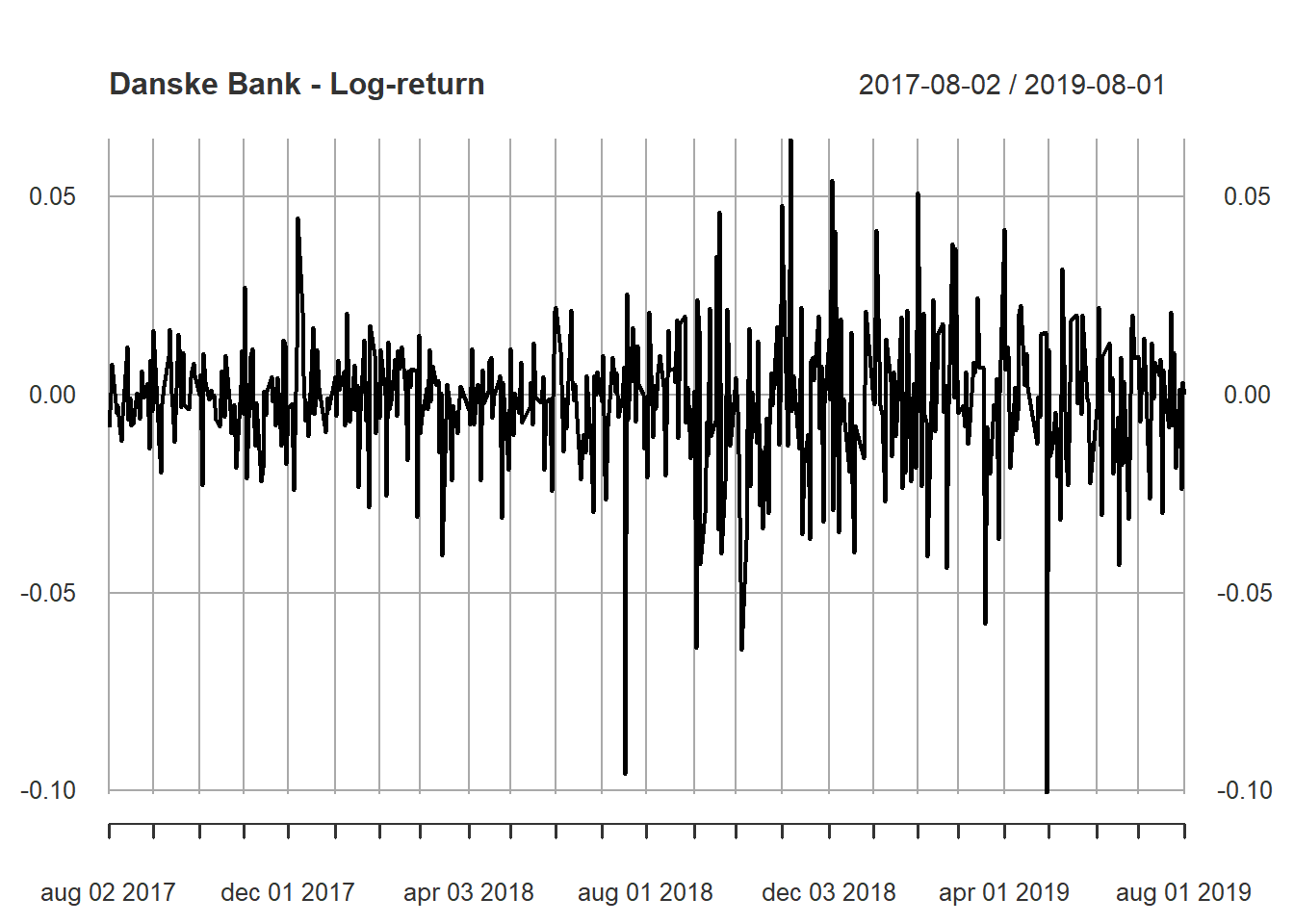
Alright. Let’s look at the data.

That’s a lot of data for a such small plot. I can’t discern for certain it stationary or not just by looking at it. Luckily, I don’t have to. Instead I run the Augmented Dickey-Fuller test on the log-returns in the next section.
Modelling
adf.test(DANSKE.CO)##
## Augmented Dickey-Fuller Test
##
## data: DANSKE.CO
## Dickey-Fuller = -8.6157, Lag order = 7, p-value = 0.01
## alternative hypothesis: stationaryAll good. If you run the code yourself, you’ll see R will tell you the p-value is lower than 0.01, which just increases the significance.
Before we proceed further the data is split into a training and testing data set. We want to compare the forecasted returns with the actual returns. Making long-term investment decisions based on a univariate time series forecast is probably not the best course of action. Instead we forecast returns for the next 12 days.
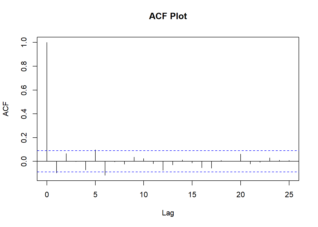
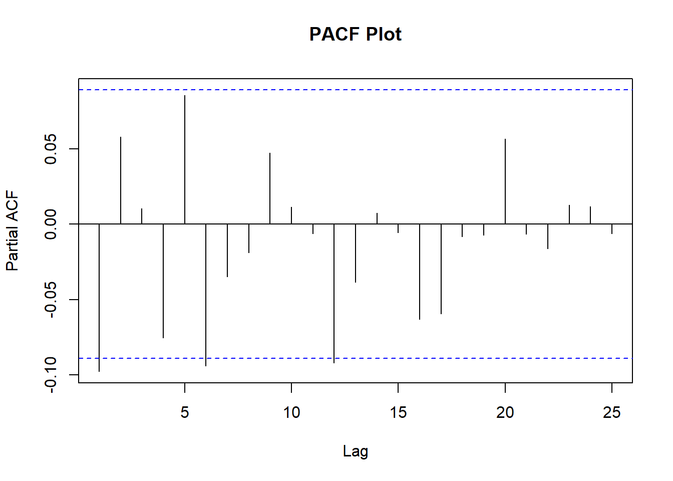
splitpoint = floor(nrow(DANSKE.CO)*((nrow(DANSKE.CO)-12)/nrow(DANSKE.CO)))To determine the parameters AR and MA for the ARIMA model we can plot the ACF (Autocorrelation Function) and PACF (Partial Autocorrelation Function).
par(mfrow = c(1,1))
acf.DANSKE = acf(DANSKE.CO[c(1:splitpoint),], main='ACF Plot', lag.max = 25)
pacf.DANSKE = pacf(DANSKE.CO[c(1:splitpoint),], main='PACF Plot', lag.max = 25)
The PACF plot can help determine the order of AR, while the ACF plot can for the order of MA terms. The highest spike of the PACF is at 1, which will be the parameter p of the ARIMA. Same is the case for the ACF plot i.e. the highest spike is at 1, which will be the parameter q of the ARIMA.
Our final ARIMA model parameters are (1, 0, 1). Since the data already was stationary no differencing is applied hence parameter d is 0.
As stated previously the forecasted returns are compared to the actual return from the testing data. The following code splits the stock data into training data set and a test data set.
DANSKE_train = DANSKE.CO[1:splitpoint]
DANSKE_test = DANSKE.CO[(splitpoint+1):nrow(DANSKE.CO)]
The ARIMA model is fitted on the training data with previously chosen parameters.
fit = arima(DANSKE_train, order = c(1, 0, 1),include.mean=FALSE)We can call a summary of a fitted model to read coefficients, standard errors etc.
summary(fit)##
## Call:
## arima(x = DANSKE_train, order = c(1, 0, 1), include.mean = FALSE)
##
## Coefficients:
## ar1 ma1
## -0.3741 0.2835
## s.e. 0.2249 0.2296
##
## sigma^2 estimated as 0.0003054: log likelihood = 1277.19, aic = -2548.38
##
## Training set error measures:
## ME RMSE MAE MPE MAPE MASE ACF1
## Training set -0.00195476 0.01747623 0.01220819 NaN Inf 0.6558061 -0.002583976The table is not very pleasant to look at with this site’s formatting, but I wasn’t able to find a better solution for now. Just by looking at the ratio between the coefficients and the standard error neither looks very significant. A simple command should confirm my suspicion.
coeftest(fit)##
## z test of coefficients:
##
## Estimate Std. Error z value Pr(>|z|)
## ar1 -0.37409 0.22489 -1.6635 0.09622 .
## ma1 0.28348 0.22960 1.2347 0.21695
## ---
## Signif. codes: 0 '***' 0.001 '**' 0.01 '*' 0.05 '.' 0.1 ' ' 1As suspected there are no significance of either variables. This will probably come even more clear when we later plot the actual returns against the forecasted returns.
The return equation from the model can be written as:
\[ y_{t}=-0.3741*y_{t-1}+0.2835*\varepsilon_{t-1} \]
Evaluating
The log returns are forecasted. We are not going to bother plot the forecasted returns for now due the size of the sample.
arima.forecast = forecast(fit, h = 12,level=99)The forecasted returns are converted to an xts-object, which is used later to plot forecasted returns vs. actual returns.
DANSKE_forecasts = xts(arima.forecast[["mean"]], order.by = index(DANSKE_test))
colnames(DANSKE_forecasts) = c("Forecasted")
The actual returns and forecasted returns are merged before it’s plotted.
DANSKE_compare = merge(DANSKE_test, DANSKE_forecasts)
colnames(DANSKE_compare) = c("Actual", "Forecasted")
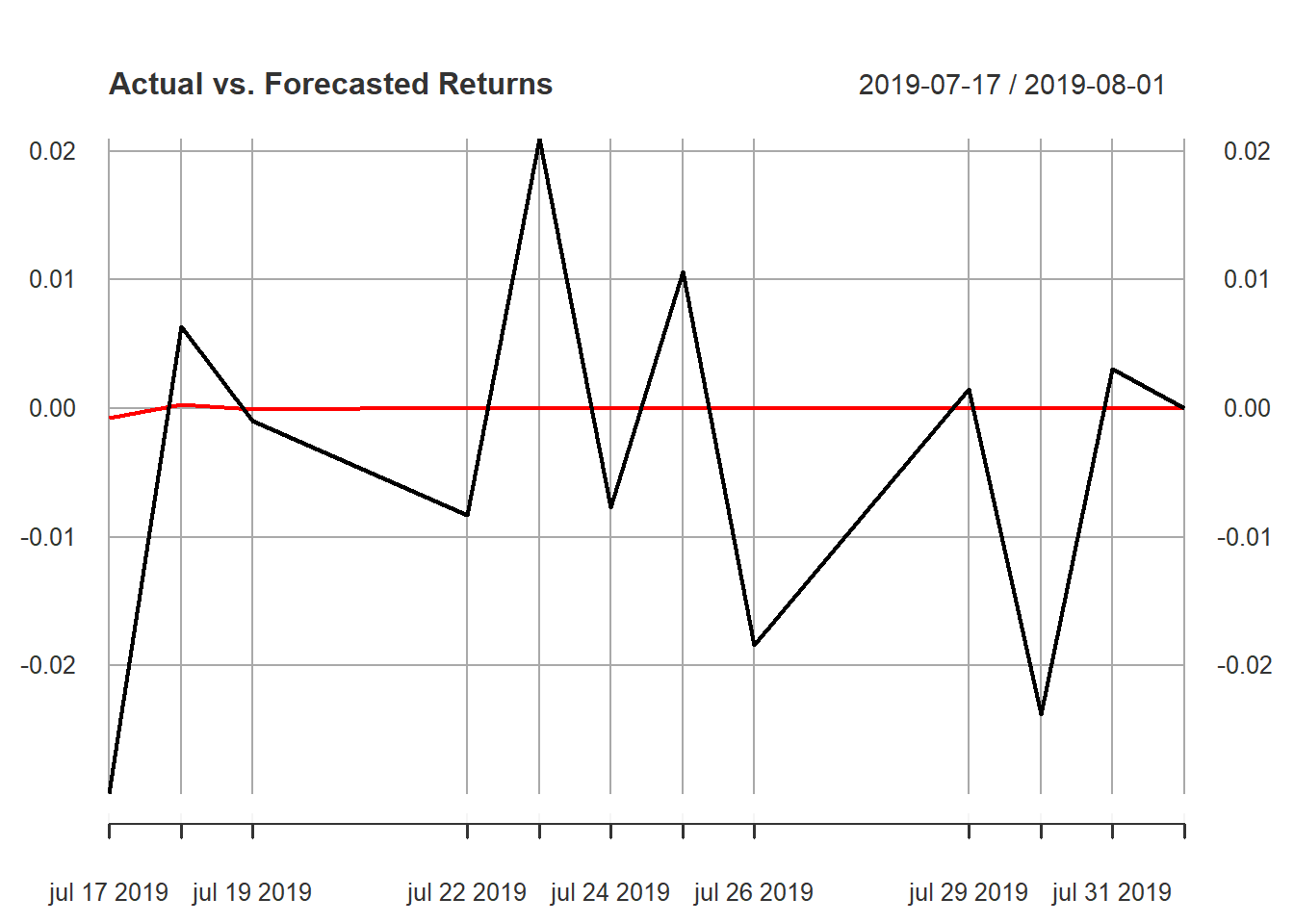
Finally, lets plot the actual returns against the forecasted returns.
plot(DANSKE_compare, main="Actual vs. Forecasted Returns")
That’s a bit underwhelming but expected. I guess this proofs the market efficiency hypothesis?
Below is a table with the accuracy of the forecast. The accuracy is binary and is determined by the sign of the actual and forecasted returns. If the signs are equal the accuracy is 1 otherwise 0. This accuracy metric leaves a lot to be desired, but let’s roll with it.
DANSKE_compare$Accuracy = sign(DANSKE_compare$Actual)==sign(DANSKE_compare$Forecasted)
print(DANSKE_compare)
## Actual Forecasted Accuracy
## 2019-07-17 -0.0299539883 -7.724654e-04 1
## 2019-07-18 0.0063554456 2.889738e-04 1
## 2019-07-19 -0.0009751147 -1.081030e-04 1
## 2019-07-22 -0.0083272388 4.044058e-05 0
## 2019-07-23 0.0209304399 -1.512853e-05 0
## 2019-07-24 -0.0077370114 5.659477e-06 0
## 2019-07-25 0.0106229682 -2.117170e-06 0
## 2019-07-26 -0.0184203080 7.920184e-07 0
## 2019-07-29 0.0014666442 -2.962884e-07 0
## 2019-07-30 -0.0238282666 1.108394e-07 0
## 2019-07-31 0.0030970403 -4.146423e-08 0
## 2019-08-01 0.0000000000 1.551148e-08 0Out of 12 days the model predicted the sign of the return correct two days. In other words, do not expect this model to gain the financial system and make you rich anytime soon.